3 Applying the PSBC model to some toy problems
We shall present the model in a simple toy problem, for illustrative purposes. As pointed out in the paper, we have to use a somewhat “bigger”" model, of the form
\[\begin{equation} \begin{split} U^{[n+1]} = U^{[n]} + \Delta_t^{u}\,f(U^{[n]},\alpha^{[n]}),\\ P^{[n+1]} = P^{[n]} + \Delta_t^{p}\,f(P^{[n]},\beta^{[n]}), \end{split}\tag{3.1} \end{equation}\]
where \(f(u,w):= u(1 - u)(u - w)\). Now, given a certain cost function that measures accuracy of the model (namely, how well it predicts in some examples) we have to train the model with respect to both variables \(\alpha^{[\cdot]}\) and \(\beta^{[\cdot]}\). What we see in (3.1) is part of what we call Phase Separation Binary Classifier (PSBC). For now, we shall see how it behaves in the 1D model; in Section 4, after many variations over this equation, we shall apply the model to the MNIST dataset.
3.1 The 1D Rectangular box problem
We shall work with a simple 1D model (the rectangular box problem), with the following labeling method:
\[\begin{equation} Y =Y(X) = \left\{\begin{array}{cc} 1, & \text{if}\quad X \geq \gamma; \\ 0, & \text{otherwise}. \end{array}\right.\tag{3.2} \end{equation}\]
folder = "Statistics/MNIST/"
with open(folder + "parameters_MNIST_Neumann.p", 'rb') as fp: data = pickle.load(fp)
### GENERATE DATA
gamma, N_data = .2, 2000
X = np.reshape(np.random.uniform(0, 1, N_data),(1, -1))
Y = np.array(X >= gamma, np.int, ndmin = 2)
### SPLIT DATA FOR CROSS VALIDATION
A, B, C, D = train_test_split(X.T, Y.T, test_size = 0.2)
#### We shall save one individual per column. We need to change that upon reading the csv later on
X_train, X_test, Y_train, Y_test = A.T, B.T, C.T, D.TIn this model, the data has to satisfy features dimension X number of elements in the sample
\(>>>\)
(1, 1600)Things go more or less as before: we define the model’s parameters,
learning_rate = (.1,.08,.93)
patience = float("inf")
sigma = .1
drop_SGD = 0.95  # See  docstring of class "Binary_phase_separation" for further information
epochs, dt, dx, eps, Nx, Nt = 600, .1, 1, 0, 1, 20
weights_k_sharing = Nt
ptt_cardnlty = 1
batch_size = None
subordinate, save_parameter_hist, orthodox_dt, with_phase = True, True, True, True
and initialize the model
Init = Initialize_parameters()

data = Init.dictionary(Nx, eps, dt, dx, Nt, ptt_cardnlty, weights_k_sharing, sigma = sigma )
data.update({'learning_rate' :  learning_rate, 'epochs' :  epochs,\
             'subordinate' :  subordinate,"patience" : patience,\
             'drop_SGD' : drop_SGD,"orthodox_dt" : orthodox_dt,'with_phase' : with_phase,
             "batch_size" : batch_size, "save_parameter_hist" : save_parameter_hist })
We are finally ready to train the model. We do so using the class Binary_Phase_Separation
Of which you can learn more about by typing
\(>>>\)
   This is the main class  of the Phase Separation Binary Classifier (PSBC).
   With its methods one can, aong other things, train the model and
   predict classifications (once the model has been trained).
If the above is not enough, you can type
\(>>>\)
Help on Binary_Phase_Separation in module binary_phase_separation object:

class Binary_Phase_Separation(builtins.object)
 |  Binary_Phase_Separation(cost=None, par_U_model=None, par_P_model=None, par_U_wrt_epochs=None, par_P_wrt_epochs=None)
 |
...
But this is maybe too much. So, let’s say that you just want to know about how to train. You can get information only about that method
\(>>>\)
        'train' method.

        This method trains the PSBC model with a given set of parameters and
        data.

        Parameters
        ----------
        X : numpy.ndarray of size Nx X N_data
            Matrix with features.
        ...
The method that we want is train. So, we do
Model.train(
    X_train, Y_train, X_train, Y_train, learning_rate, dt, dx, Nt,\
        weights_k_sharing, eps = eps, epochs = epochs, \
        subordinate = subordinate, with_phase = with_phase,\
        drop_SGD = drop_SGD, sigma = sigma,\
        orthodox_dt = orthodox_dt, print_every = 300,\
            save_parameter_hist = save_parameter_hist
)
\(>>>\)
 epoch : 0 cost 0.11494985702898435

 accuracy : 0.70375

 epoch : 300 cost 0.022553932287346947

 accuracy : 0.9775
If you want to take a look at how the cost function behaves over epochs, you can plot it (see full code in Notebook_examples.ipynb). The output is given below.
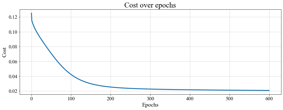
The evolution of the cost over epochs, for the 1D PSBC model with labeling (3.2).
And if you want to take a look at the behavior of the set \(\mathscr{P}_{\alpha}\) you can also do. Just type
which will give you a dictionary with two keys: “U” and “P”
\(>>>\)
dict_keys(['P', 'U'])They concern the behavior of trainable weights for the U variable, and for the P variable. They can be plotted as
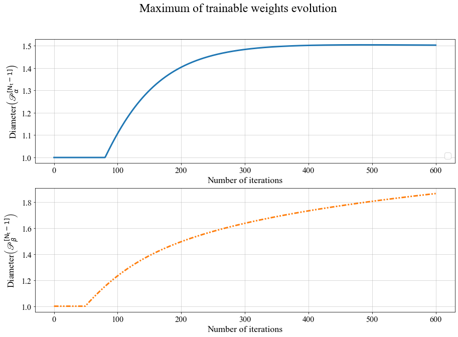
The evolution of the diameters \(\mathrm{\mathscr{P}_{\alpha}}\) and \(\mathrm{\mathscr{P}_{\beta}}\) over epochs, for the 1D PSBC model with labeling (3.2).
This is the typical behavior of these quantities: they remain constant (equal to 1) up to a certain point, to then grow in a logarithmic shape. Note that the point of departure from the value 1 is different for both variables; that’s because both quantities \(\Delta_t^u\) and \(\Delta_t^p\) in (3.1) are allowed to vary independently (see the paper for further information).
We can also check the behavior of accuracythroughout epochs:
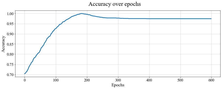
The evolution of accuracy over epochs, for the 1D PSBC modelwith labeling (3.2).
Note the the model peaks (reaches a point of high accuracy) before the final epoch. This natural “deterioration” is what lead researchers to design Early Stopping methods; cf. (Prechelt 1998). We can in fact know what that epoch was by typing
\(>>>\) array(181)
which is before final epoch - in this case, 600. The accucary (for the training set) at epoch 181 was
\(>>>\) array(1.)
that is, 100% accuracy. If you want to retrieve the model parameters at such an epoch you just need to type
which will give the value of the parameters used when the model achieved its best performance.
For this simple model we did something else: we are saving all the parameters in the model at each epoch.1
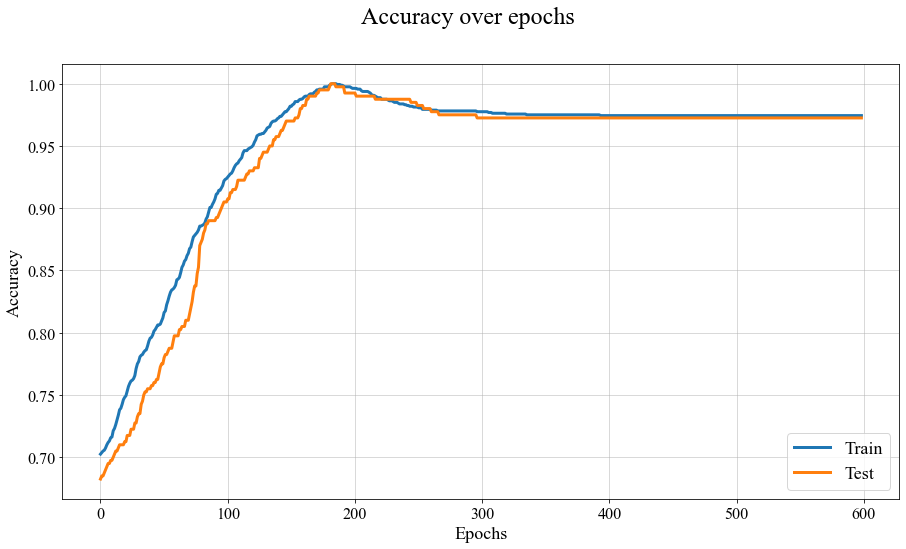
Evolution of accuracy for train and test set over epochs, for the 1D PSBC problem with labeling (3.2).
References
Prechelt, Lutz. 1998. “Early Stopping - but When?” In Neural Networks: Tricks of the Trade, edited by Müller Orr Genevieve B., 55–69. Berlin, Heidelberg: Springer Berlin Heidelberg. https://doi.org/10.1007/3-540-49430-8_3.
It is clear that whenever one deals with big models memory is an impeditive obstruction to reproducing this; in such a case, it is better to set “save_parameter_hist = False” in order to save memory.↩︎