4 The MNIST database

The MNIST database is a well known database of handwritten digits used in the classical paper (Lecun et al. 1998). In this project we only used (suggestively) the subset of digits “0” and “1”, for we are doing binary classification only.

### READ MNIST DATASET TO PANDAS DATAFRAME AND THEN TO NUMPY FILE
data_train_MNIST = pd.read_csv('Examples/data_train_normalized_MNIST.csv')
data_test_MNIST = pd.read_csv('Examples/data_test_normalized_MNIST.csv')

X_train_MNIST = (data_train_MNIST.iloc[:,:-1]).to_numpy()
Y_train_MNIST = np.reshape(data_train_MNIST.iloc[:,-1].to_numpy(), (1,-1))
X_test_MNIST = (data_test_MNIST.iloc[:,:-1]).to_numpy()
Y_test_MNIST = np.reshape(data_test_MNIST.iloc[:,-1].to_numpy(), (1,-1))

X_train_MNIST, X_test_MNIST = X_train_MNIST.T , X_test_MNIST.T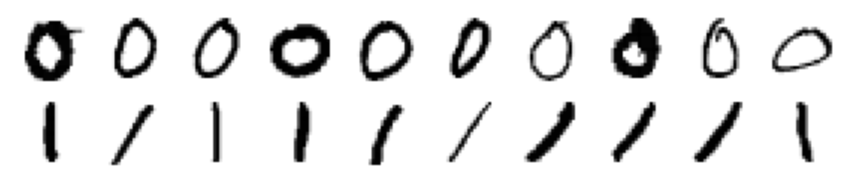

A subsample of digits “0” and “1” in the MNIST database.

One can also visualize the trainable weights as heatmaps (see full code in Notebook_examples.ipynb).

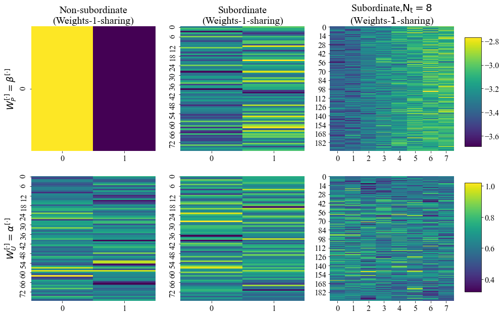
Heatmaps of trainable weights for some trained PSBC models in the Examples folder.

4.1 Retrieving some statistics

To get a flavor of what is in the statistics folder, we first need to retrieve some of this data:

parameters_MNIST_nondif, stats_folder_MNIST = {}, "Statistics/MNIST/"
with open(stats_folder_MNIST + "parameters_MNIST_nondif.p", 'rb') as fp: 
    parameters_MNIST_nondif = pickle.load(fp)

parameters_MNIST_Neumann, stats_folder_MNIST = {}, "Statistics/MNIST/"
with open(stats_folder_MNIST + "parameters_MNIST_Neumann.p", 'rb') as fp:
        parameters_MNIST_Neumann = pickle.load(fp)

parameters_MNIST_Periodic, stats_folder_MNIST = {}, "Statistics/MNIST/"
with open(stats_folder_MNIST + "parameters_MNIST_Periodic.p", 'rb') as fp:
        parameters_MNIST_Periodic = pickle.load(fp)

The function accuracies is part of the module aux_fnts_for_jupyter_notebooks.py, which is available in this Github (Monteiro 2020 b). As before, help on this equation can be called typing ‘help(accuracies)’.

With data in the Statistics folder we can plot the graph of accuracies of the non-diffusive PSBC for different values of partition cardinality \(\mathrm{N_{ptt}}\).

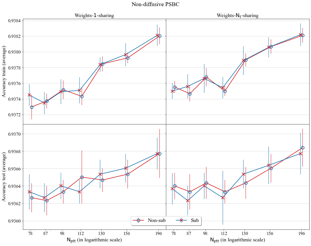
A comparison of average accuracy of the non-diffusive PSBC for different values of Partition cardinality; models compared either have subordinate phase (tagged as “Sub”) or not (non-subordinate phase, tagged as “Non-sub”).

If can also see the evolution of the maximum of trainable weights over epochs, for a Periodic PSBC with \(\mathrm{N_t} =1\).

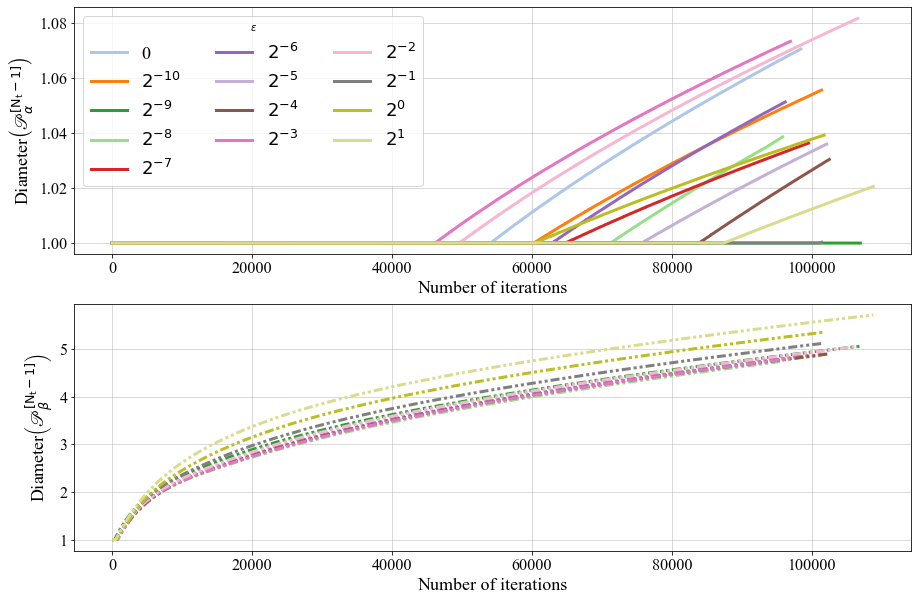
The behavior of \(\mathscr{P}_{\alpha}^{[\cdot]}\) and \(\mathscr{P}_{\beta}^{[\cdot]}\) over time, for a Periodic PSBC with \(\mathrm{N_t} =1\).

With these data we can also plot confusion matrices.

parent_folder = "Examples/"
folder_now = parent_folder + "W1S-Nt8/simulation1/"
with open(folder_now + "Full_model_properties.p", 'rb') as fp: Full_model_properties = pickle.load(fp)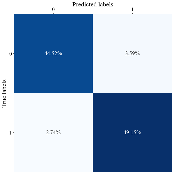

Confusion matrix of a realization of the diffusive PSBC with Neumann BCs, weights-1-sharing, and \(\mathrm{N_t = 8}\).

There are other things that we do as well: for instance, we can plot Table 4 in the Supplement, which shows the average value of the maximum (in \(\ell^{\infty}\)-norm) of trainable weights of non-diffusive PSBC models for different values of partition cardinality \(\mathrm{N_t}\).

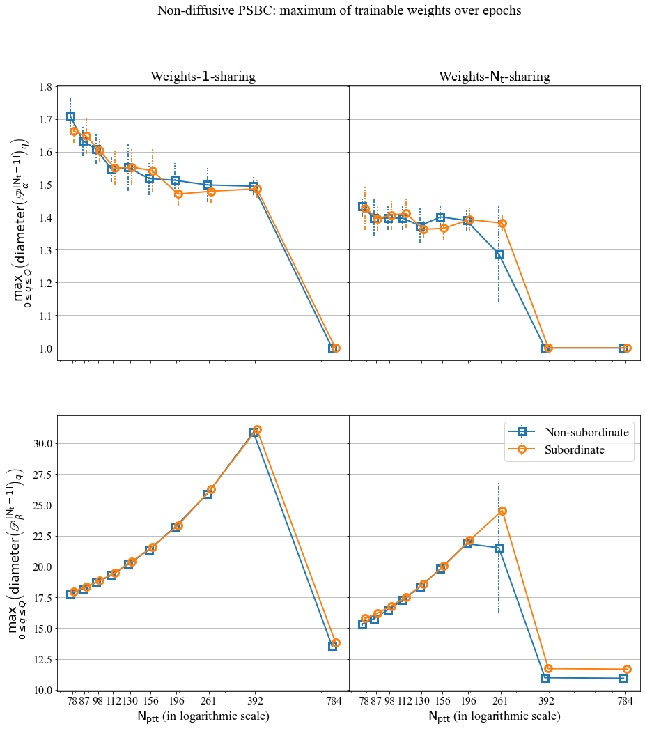
The maximum over epochs. You find the code for this plot in Notebook_examples.ipynb.

4.2 A “homemade” example: hadwritten 0 and 1

We now step foward to a higher dimensional feature space, using equations that are similar to those shown in Section 3 of this tutorial. There is an interesting interplay between high-dimensionality of feature spaces and model compressibility, which we highlight here by applying the PSBC to the subset “0”-“1” of the MNIST database; we once more refer the reader to Sections 4 and 5 in the paper for more details.

The goal in this section is to illustrate a bit more of the PSBC’s use by predicting the label for some of the author’s own handwritten numbers. For that we shall use the trainable models available in (Monteiro 2020 a), in the tarball PSBC_Examples.tar.gz. Two of these digits are shown below.

Two of the author’s own handwritten numbers; original photo, treated using Gimp.

In fact, we shall use 6 of the author’s handwritten digits - 3 zeros, 3 ones - for this notebook. If you read the first papers of LeCun et al. about the MNIST project, there is a description of the way pictures were taken (see for instance, Section III A in (Lecun et al. 1998), or the explanation in LeCun’s MNIST webpage), so that they look the way they do in cell 36 of Notebook_examples.ipynb: the images had to be controlled for angle, centralization, etc; this is part of the statistical design, which I tried to follow here without too much concern (because this is just a tutorial) but, somehow, “as close as possible”.

Pictures we cropped using GIMP, a free software for image manipulation: you take a picture, crop it, go to image, set it into grayscale, adjust for light contrast and other things. And that’s it.

Now, with them cropped, “MNIST-like” grayscale images in hands, you proceed as in the next cell, reshaping these pictures as a 28 x 28 matrix. We show what the two digits that you saw before will look like.

from PIL import Image

def create_MNIST_type_figure(name):
    """Convert jpg figure to a (28,28) numpy array"""
    image = Image.open(name).convert('L')
    image2 = image.resize((28,28))
    im2_as_array = 255- np.array(image2,  dtype=np.uint8)
    print("image has shape", im2_as_array.shape)

    return im2_as_array

my_0 = create_MNIST_type_figure("figures/my_0.jpg")
my_0_v2 = create_MNIST_type_figure("figures/my_0_v2.jpg")
my_0_v3 = create_MNIST_type_figure("figures/my_0_v3.jpg")
my_1 = create_MNIST_type_figure("figures/my_1.jpg")
my_1_v2 = create_MNIST_type_figure("figures/my_1_v2.jpg")
my_1_v3 = create_MNIST_type_figure("figures/my_1_v3.jpg")

fig, ax = plt.subplots(1,2)
ax[0].imshow(my_0, cmap='binary')
ax[1].imshow(my_1, cmap='binary')
ax[0].axis(False)
ax[1].axis(False)
plt.show()

You will get this

The handwritten digits shown above, now as 28X28 pixels images.

Recall that we need to flatten these matrices,

my_0_for_psbc = my_0.flatten(order='C')
...

and we can then combine all these 6 flattened images as columns in a single matrix combined_handwritten, whose size is \(784\times 6\).

Now we initialize the PSBC model

with open("Examples/W1S-Nt8/simulation1/Full_model_properties.p", 'rb') as fp: load_mnist = pickle.load(fp)

psbc_testing = Binary_Phase_Separation()

and apply to our matrix/data combined_handwritten with the trained weights we have chosen.

prediction = psbc_testing.predict(combined_handwritten, load_mnist["best_par_U_model"],load_mnist["best_par_P_model"])
print(prediction)

…and we fail, as we see in the output below. Floating number overflows, “NAN”, etc.. sad news..

\(>>>\)

[0 0 0 0 0 0]

/Users/rafaelmonteiro/Desktop/PSBC/All_cases/binary_phase_separation.py:475: RuntimeWarning: overflow encountered in multiply
  v = v +  dt * v * (1-v) * (v-alpha_x_t)
/Users/rafaelmonteiro/Desktop/PSBC/All_cases/binary_phase_separation.py:477: RuntimeWarning: invalid value encountered in matmul
  v = np.matmul(Minv,v)
/Users/rafaelmonteiro/Desktop/PSBC/All_cases/binary_phase_separation.py:1128: RuntimeWarning: invalid value encountered in greater
  keepdims = True, axis = 0))) > .5, dtype = np.int32)

This seems really bad… but do not despair: recall that data need to satisfy the normalization conditions: all the features have to be in the range \([0,1]\). We are in fact very far from that now: if you look for the minimum and maximum value of these matrices you will get \(0\) and \(255\), respectively, as an answer.

With that said, let’s normalize the data:

init_data = Initialize_Data()

So, the data get’s normalized, but centered. By default, it gets rescaled in the range [0.4,0.6]. What we do then is: (i) we normalize it, then (ii) we add 0.1 to it.

combined_handwritten_for_psbc, _, _ = init_data.normalize(combined_handwritten)
combined_handwritten_for_psbc = 0.1+ combined_handwritten_for_psbc

Now we are in better shape: if you look for minimum and maximum of the matrix \(combined\_handwritten\_for\_psbc\) you will get \(0.5\) and \(0.7000000000000001\).

Some of the author’s handwritten examples for this tutorial.

Now let’s see how well the PSBC does in predicting them (note that, for the subset “0” and “1” of the MNIST database we already know that all these model perform quite well, separating these two classes with accuracy about 94%).

for name in ["W1S-NS", "W1S-S", "WNtS-NS", "WNtS-S",\
            "W1S-Nt2", "W1S-Nt4", "W1S-Nt8",\
             "WNtS-Nt1","WNtS-Nt2", "WNtS-Nt4", "WNtS-Nt8",\
             "Per_W1S-Nt2", "Per_W1S-Nt4", "Per_W1S-Nt8",\
             "Per_WNtS-Nt1","Per_WNtS-Nt2", "Per_WNtS-Nt4", "Per_WNtS-Nt8"]:
            
    with open("Examples/"+name+"/simulation1/Full_model_properties.p", 'rb') as fp:
        load_mnist = pickle.load(fp)
    
    psbc_testing = Binary_Phase_Separation()
    prediction = \
    psbc_testing.predict(
        combined_handwritten_for_psbc,  load_mnist["best_par_U_model"], load_mnist["best_par_P_model"],\
        subordinate = load_mnist["best_par_U_model"]["subordinate"]
    )
    print("Model", name, " predicts", np.squeeze(prediction), "and correct is, [0 0 0 1 1 1]" )

\(>>>\)

Model W1S-NS  predicts [0 0 0 0 1 1] and correct is, [0 0 0 1 1 1]
Model W1S-S  predicts [0 0 0 0 1 1] and correct is, [0 0 0 1 1 1]
Model WNtS-NS  predicts [0 0 0 0 1 1] and correct is, [0 0 0 1 1 1]
Model WNtS-S  predicts [0 0 0 0 1 1] and correct is, [0 0 0 1 1 1]
Model W1S-Nt2  predicts [0 0 0 0 1 1] and correct is, [0 0 0 1 1 1]
Model W1S-Nt4  predicts [0 0 0 0 1 1] and correct is, [0 0 0 1 1 1]
Model W1S-Nt8  predicts [0 0 0 0 1 1] and correct is, [0 0 0 1 1 1]
Model WNtS-Nt1  predicts [0 0 0 0 1 1] and correct is, [0 0 0 1 1 1]
Model WNtS-Nt2  predicts [0 0 0 0 1 1] and correct is, [0 0 0 1 1 1]
Model WNtS-Nt4  predicts [0 0 0 0 1 1] and correct is, [0 0 0 1 1 1]
Model WNtS-Nt8  predicts [0 0 0 0 1 1] and correct is, [0 0 0 1 1 1]
Model Per_W1S-Nt2  predicts [0 0 0 0 1 1] and correct is, [0 0 0 1 1 1]
Model Per_W1S-Nt4  predicts [0 0 0 0 1 1] and correct is, [0 0 0 1 1 1]
Model Per_W1S-Nt8  predicts [0 0 0 0 1 1] and correct is, [0 0 0 1 1 1]
Model Per_WNtS-Nt1  predicts [0 0 0 0 1 1] and correct is, [0 0 0 1 1 1]
Model Per_WNtS-Nt2  predicts [0 0 0 0 1 1] and correct is, [0 0 0 1 1 1]
Model Per_WNtS-Nt4  predicts [0 0 0 0 1 1] and correct is, [0 0 0 1 1 1]
Model Per_WNtS-Nt8  predicts [0 0 0 0 1 1] and correct is, [0 0 0 1 1 1]

It is getting all correct, except for the 4th picture (which is in fact the way that I usually write, with that huge horizontal “foot”).

References

Lecun, Yann, Léon Bottou, Yoshua Bengio, and Patrick Haffner. 1998. “Gradient-Based Learning Applied to Document Recognition.” In Proceedings of the Ieee, 2278–2324.

Monteiro, Rafael. 2020a. “Data Repository for the Paper ‘Binary Classification as a Phase Separation Process’.” Zenodo Repository. https://dx.doi.org/10.5281/zenodo.4005131; Zenodo. https://doi.org/10.5281/zenodo.4005131.

Monteiro, Rafael. 2020b. “Source Code for the Paper ‘Binary Classification as a Phase Separation Process’.” GitHub Repository. https://github.com/rafael-a-monteiro-math/Binary_classification_phase_separation; GitHub.