2 Nonlinear diffusion equations: a numerical example
As discussed in Section 1.1 in the paper, the nonlinear diffusion processes are in the backdrop of this model. The heart of the model is the Allen-Cahn equation (Fife 1979),(Aronson and Weinberger 1978),(Allen and Cahn 1979), a well-known equation in the field of pattern formation. Just to show how part of the PSBC’s implementation can be used to evolve an initial boundary value problem with Neumann boundary conditions: we shall take
\[\begin{equation} u_0(x) = \frac{1- \sin(\pi(2x - 1))}{2}\tag{2.1} \end{equation}\]
as an initial condition to the Allen-Cahn equation
\[\begin{equation} \partial_tu(x, t) = \varepsilon^2 \partial_x^2u(x, t) + u(x, t)(1 - u(x, t))(u(x, t) - \alpha(x)).\tag{2.2} \end{equation}\]
The parameter \(\alpha(\cdot)\) embodies medium heterogeneity. In the case shown here, we choose \(\alpha(x) = -2\), when \(x <0.5\), and \(\alpha(x)\) = 2, when \(x \geq 0.5\).
When we plot the evolution of \(u_0(\cdot)\) through the Allen-Cahn equation as a surface, we get the plot below.
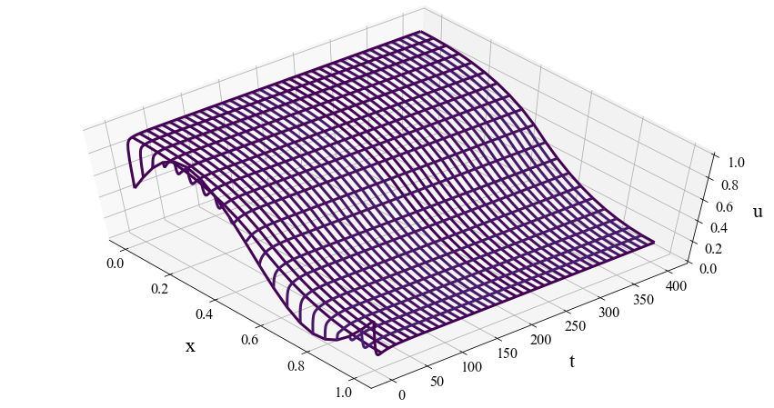
The initial condition \(u_0(\cdot)\) shown in Equation (2.1), as it evolves according to the Allen-Cahn equation (2.2).
Actually, we shall mostly treat the coefficients of this PDE as trainable weights: parameters that we will tweak in order to get the desired asymptotic behavior and, in this way, do binary classification. This is what we explain next.
One of the first motivations to this project can be found in the interesting paper (Angenent, Mallet-Paret, and Peletier 1987), where they have shown that several nontrivial layered patterns^{Stationary solutions to equation (2.2) that, roughly speaking, gets “concentrated” around values 0 and 1, displaying layers in between these values.} can be found if \(\alpha(\cdot)\) is non-homogeneous in space. There is an extensive discussion about why this is interesting, and we refer the reader to Section 1.1 in the paper.
Remark: You can read more about pattern formation in the book (Nishiura 2002) (Chapter 4.2 deals with the Allen-Cahn model), and also in the very nice article Arnd Scheel wrote to the Princeton Companion to Applied Mathematics, Section IV. 27 (Dennis et al. 2015).
2.1 Propagation with randomly generated coefficients
Next, for illustrative purposes, we would like to evolve and plot the evolution of several different initial conditions in the interval [0,1] (this is not shown in the paper, but the code can be found in version 1 of this project, in “Notebook_examples.ipynb”). The model that we use is, initially, a discretization of (2.2), with \(\varepsilon = 0\), which then becomes an ODE:
\[\begin{equation} U^{[n+1]} = U^{[n]} + \Delta_t^{u}f(U^{[n]},\alpha^{[n]}),\tag{2.3} \end{equation}\]
where \(f(U^{[n]},\alpha^{[n]}):= U^{[n]}(1 - U^{[n]})(U^{[n]} - \alpha^{[n]} )\).
It is good to have in mind that the coefficients in the above ODE will play the role of trainable weights in Machine Learning: we will “adjust” the coefficients in \(\alpha(\cdot)\) in order to achieve a certain final, target end state.
As mentioned earlier, there is a clear correspondence between the initial value (ODE/PDE) problem and forward propagation and, consequently, the stability of (2.3) has to be considered. The discretization it presents is known as (explicit) Euler method, which is known to be (linearly) unstable in many cases. A good part of the paper was devoted to showing that there is some kind of nonlinear stabilization mechanism that prevents solutions from blowing up, a condition referred to as Invariant Region Enforcing Condition, which establishes a critical threshold for the size of \(\Delta_t^u\), beyond which solutions can blow up.
To get this critical value for \(\Delta_t^u\) it is necessary to quantify
\[\begin{equation} \max_{1\leq k \leq \mathrm{N_t}}\max\{1,\vert \alpha^{[k]}\vert\} <+\infty,\tag{2.4} \end{equation}\]
based on which we adjust the parameter \(\Delta_t^u\) accordingly, in a nontrivial way.1 In result, the evolution of \(U^{[\cdot]}\) does not end up in a floating point overflow (in other words, a blow up in \(\ell^{\infty}\) norm).
We set up a little experiment, where in some we obey the Invariant Region Enforcing Condition, and in some we don’t. We take several initial condition on the interval \([0,1]\) and evolving them according to (2.3).
As discussed in the Appendix A in the paper, the PSBC randomly initializes trainable weights coefficients as realizations of a Normal random variable with average 0.5 and variance 0.1. We set them as uniform random variables in the interval [0,1], which implies that the left hand side of (2.4) is bounded by 1.
We obtain the following figure.
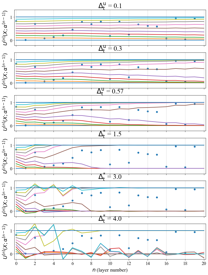
The evolution of initial conditions in the interval \([0,1]\) through the Allen-Cahn-equation (2.2) with \(\varepsilon = 0\) (that is, an ODE) in 1D, with coefficients given by random coefficients generated as an uniform distribution in the interval \([0,1]\).
In this figure we can observe that for small values of \(\mathrm{\Delta_{t}^u}\) the orbits obey some monotonic behavior. Of course, existence and uniqueness theorems in ODE guarantee that at the continuum level, but translating such property to the discrete model is far different: in fact, in many cases this property do not hold. The reasoning behind the existence of critical values of \(\mathrm{\Delta_{t}^u}\) under which the solution is “well behaved” (that is, the solution is always bounded) goes back to the idea of Invariant regions, exploited extensively in PDEs: we refer the reader to Chapter 14 in (Smoller 1994); if you want to see how it applies in the discrete setting, especially in finite-difference schemes for reaction diffusion models, see (Hoff 1978) and the Appendix C of the paper).
Remark: in spite of being a Recursive Neural Network (RNN) type of model, there are considerable differences. Indeed, RNN’s parameters are adjusted with the unique intention of optimizing a cost function, whereas in the PSBC we adjust \(\mathrm{\Delta_{t}^u}\) in order to tame the growth of evolved features through forward propagation. We address the similarities in Section 4 of the paper.
References
Allen, Samuel M, and John W Cahn. 1979. “A Microscopic Theory for Antiphase Boundary Motion and Its Application to Antiphase Domain Coarsening.” Acta Metallurgica 27 (6): 1085–95.
Angenent, S. B., J. Mallet-Paret, and L. A. Peletier. 1987. “Stable Transition Layers in a Semilinear Boundary Value Problem.” J. Differential Equations 67 (2): 212–42. https://doi.org/10.1016/0022-0396(87)90147-1.
Aronson, D. G., and H. F. Weinberger. 1978. “Multidimensional Nonlinear Diffusion Arising in Population Genetics.” Adv. In Math. 30 (1): 33–76. https://doi.org/10.1016/0001-8708(78)90130-5.
Dennis, Mark R., Paul Glendinning, Paul A. Martin, Fadil Santosa, and Jared Tanner, eds. 2015. The Princeton Companion to Applied Mathematics. Princeton University Press, Princeton, NJ. https://doi.org/10.1515/9781400874477.
Fife, Paul C. 1979. Mathematical Aspects of Reacting and Diffusing Systems. Vol. 28. Lecture Notes in Biomathematics. Springer-Verlag, Berlin-New York.
Hoff, David. 1978. “Stability and Convergence of Finite Difference Methods for Systems of Nonlinear Reaction-Diffusion Equations.” SIAM J. Numer. Anal. 15 (6): 1161–77. https://doi.org/10.1137/0715077.
Nishiura, Yasumasa. 2002. Far-from-Equilibrium Dynamics. Vol. 209. Translations of Mathematical Monographs. American Mathematical Society, Providence, RI.
Smoller, Joel. 1994. Shock Waves and Reaction-Diffusion Equations. Second. Vol. 258. Grundlehren Der Mathematischen Wissenschaften [Fundamental Principles of Mathematical Sciences]. Springer-Verlag, New York. https://doi.org/10.1007/978-1-4612-0873-0.
Because, of course, \(\Delta_t^u =0\) also does the job, but does not deliver what we want.↩︎